
본 게시글은 필자가 강의, 책을 통해 학습하며 개인적으로 정리한 것으로 오류가 있을 수 있습니다.
또한 본문의 모든 정보는 최하단 출처를 기반으로 작성되었습니다.
로지스틱 회귀를 실제로 구현해보자.
Training Data는 다음과 같다.
x(x1, x2) = [[1,2],[2,3],[3,1],[4,3],[5,3],[6,2]]
y = [[0],[0],[0],[1],[1],[1]]
전체 코드
import tensorflow as tf

x_data = [[1, 2],
          [2, 3],
          [3, 1],
          [4, 3],
          [5, 3],
          [6, 2]]
y_data = [[0],
          [0],
          [0],
          [1],
          [1],
          [1]]

tf.model = tf.keras.Sequential()
tf.model.add(tf.keras.layers.Dense(units=1, input_dim=2))
# use sigmoid activation for 0~1 problem
tf.model.add(tf.keras.layers.Activation('sigmoid'))

'''
better result with loss function == 'binary_crossentropy', try 'mse' for yourself
adding accuracy metric to get accuracy report during training
'''
tf.model.compile(loss='binary_crossentropy', optimizer=tf.keras.optimizers.SGD(lr=0.01), metrics=['accuracy'])
tf.model.summary()

history = tf.model.fit(x_data, y_data, epochs=5000)

# Accuracy report
print("Accuracy: ", history.history['accuracy'][-1])
Linear Regression에서 다룬 예제의 코드와 비슷하다.
tf.model = tf.keras.Sequential()
tf.model.add(tf.keras.layers.Dense(units=1, input_dim=2))
# use sigmoid activation for 0~1 problem
tf.model.add(tf.keras.layers.Activation('sigmoid'))
Layer의 Activation fuction은 sigmoid로 지정했다.
로지스틱 회귀 개념 학습에서 언급한바와 같이 sigmoid함수는 이진 분류 모델에 주로 사용된다.
이전에는 이 활성화 함수에 대해서 언급하지 않았으므로 한 번 짚고 넘어가자.
activation fuction이란 현재 layer로 들어오는 input nodes에서 next Layer로 넘어가는 output nodes 사이의
'Mathematical gate'이다.
조금 더 구체적인 정보는 아래 링크를 참고하자.
7 Types of Activation Functions in Neural Networks: How to Choose?
Understand the evolution of different types of activation functions in neural network and learn the pros and cons of linear, step, ReLU, PRLeLU, Softmax and Swish.
missinglink.ai
tf.model.compile(loss='binary_crossentropy', optimizer=tf.keras.optimizers.SGD(lr=0.01), metrics=['accuracy'])이전의 Linear Regression에서 loss fuction으로 대표적인 MSE를 사용했다면,
Logistic Classification에서는 Binary Crossentropy를 사용한다.
이는 Logistic Regression개념 포스팅에서 언급한 log함수를 사용한 cost func계열이라 생각하면 된다.
또한, compile의 metrics인자로 accuracy를 지정한 모습을 볼 수 있다.
metrics는 모델의 학습으로 부터 측정하고자 하는 기준이다.(사용 이유에 대해 잘 정리된 답변을 참고하자.)
(참고용)
Tensorflow version 1.x
import tensorflow as tf

x_set = [[1,2],[2,3],[3,1],[4,3],[5,3],[6,2]]
y_set = [[0],[0],[0],[1],[1],[1]]

X = tf.placeholder(tf.float32, shape=[None,2])
Y = tf.placeholder(tf.float32, shape=[None,1])

w = tf.Variable(tf.random_normal([2,1]), name='weight')
b = tf.Variable(tf.random_normal([1]), name='bias')

# hypothesis for Logistic Regression
hypothesis = tf.sigmoid(tf.matmul(X,w) + b)

# cost func for Logistic Regression
cost = -tf.reduce_mean(Y*tf.log(hypothesis) + (1-Y)*tf.log(1-hypothesis))

train = tf.train.GradientDescentOptimizer(learning_rate=0.01).minimize(cost)

# using cast for Classification
predicted = tf.cast(hypothesis > 0.5, dtype=tf.float32)
accuracy = tf.reduce_mean(tf.cast(tf.equal(predicted, Y), dtype=tf.float32))

with tf.Session() as sess:
    sess.run(tf.global_variables_initializer())

    for step in range(10001):
        cost_, _ = sess.run([cost,train], feed_dict={X: x_set, Y: y_set})
        if step % 200 == 0:
            print(step, cost_)

    h, c, a = sess.run([hypothesis, predicted, accuracy], feed_dict={X: x_set, Y: y_set})
    print("\nHypothesis: ", h, "\nCorrect(Y): ", c, "\nAccuracy: ", a)
대부분 코드는 Linear Regression의 예제와 비슷하므로 설명은 생략한다.
잘 만들어진 cost function에 경사하강법을 사용하여 cost를 최소화 한 뒤,
직관적으로 1과 0으로 분류 된 우리의 prediction과 이에 대한 accuracy를 확인하기 위해 casting 을 사용하였다.
tf.cast : 입력한 조건과 data type에 따라 tensor를 해당 dtype으로 알맞게 변환 시켜준다.
(위의 경우 prediction은 hypothesis가 0.5 보다 크면 1(Pass), 작으면 0(Fail)로 casting,
accuracy는 prediction과 training set의 결과가 일치하면 1(True), 그렇지 않으면 0(False)로 casting)
결과는 다음과 같다.
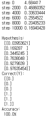
단순한 예제라 정확도는 100%가 나온다.
참고 문헌 및 자료
1. Sung Kim Youtube channel : https://www.youtube.com/channel/UCML9R2ol-l0Ab9OXoNnr7Lw
Sung Kim
컴퓨터 소프트웨어와 딥러닝, 영어등 다양한 재미있는 이야기들을 나누는 곳입니다.
www.youtube.com
2. Andrew Ng Coursera class : https://www.coursera.org/learn/machine-learning
3. 조태호(2017). 모두의 딥러닝. 서울: 길벗
'IT study > 모두를 위한 딥러닝' 카테고리의 다른 글
| Softmax Regression(2) - ex.1 (0) | 2020.08.10 |
|---|---|
| Softmax Regression(1) (0) | 2020.08.05 |
| Logistic Regression(1) (0) | 2020.08.03 |
| Reading csv Files in tensorflow(+ using google colab) (0) | 2020.07.29 |
| Linear Regression(4) - ex.2 (0) | 2020.07.29 |